2 Plots Python
Posted : admin On 4/3/2022The line chart is used to display the information as a series of the line. Our recommended IDE for Plotly's Python graphing library is Dash Enterprise's Data Science Workspaces, which has both Jupyter notebook and Python code file support. Find out if your company is using Dash Enterprise. Do you know the box plot? Wikipedia defines the box plot as a method for.
Plotting pairwise data relationships¶. PairGrid also allows you to quickly draw a grid of small subplots using the same plot type to visualize data in each. In a PairGrid, each row and column is assigned to a different variable, so the resulting plot shows each pairwise relationship in the dataset.This style of plot is sometimes called a “scatterplot matrix”, as this is the most. Semilog Plot¶ Semilog plots are the plots which have y-axis as log-scale and x-axis as linear.
Matplotlib is a Python 2-d and 3-d plotting library which producespublication quality figures in a variety of formats and interactiveenvironments across platforms. Matplotlib can be used in Python scripts, thePython and IPython shell, web application servers, and six graphical userinterface toolkits.
Documentation
The matplotlib documentation is extensive and covers all the functionality indetail. The documentation is littered with hundreds of examples showing a plot and theexact source code making the plot:
- Matplotlib home page: key plotting commands in a table
- Pyplot tutorial: intro to 1-D plotting
- Interactive navigation: how to use the plot window for zooming etc.
- Screenshots: screenshots and code for about 20 key types of matplotlib functionality
- Thumbnail gallery: hundreds of thumbnails (find a plot like the one you want to make)
- Text intro: manipulate text
- Mathematical expressions:put math in figure text or labels
- FAQ: FAQ, including a useful Howto section (e.g. multiple y-axis scales, make plot aspect ratio equal, etc)
- Search: find documentation for specific functions or general concepts
- Customizing matplotlib: making itbeautiful and well-behaved
- Line2D: knobs to twiddle for customizing a line or points in a plot
Hints on getting from here (an idea) to there (a publishable plot)
- Start with Screenshots for the broadplotting capabilities
- Go to the thumbnail gallery and scan the thumbnails tofind something similar.
- Googling is unfortunately not the best way to get to the detailed help forparticular functions. For example googling “matplotlib errorbar” just gives the home page and thepyplot API docs. The
errorbar()function is then not so easy to find. - Instead use Search andenter the function name. Most of the high-level plotting functions are inthe
pyplotmodule and you can find them quickly by searching forpyplot.<function>, e.g.pyplot.errorbar. - When you are ready to put your plot into a paper for publicationsee the page on Publication-quality plots.
Plotting 1-d data
The matplotlib tutorial on Pyplot (Copyright (c)2002-2009 John D. Hunter; All Rights Reserved and license) is an excellentintroduction to basic 1-d plotting. The content below has been adapted from the pyplottutorial source with some changes and the addition of exercises.
Basic plots
So let’s get started with plotting using a standard startup idiom that will workfor both interactive and scripted plotting. In this case we are workinginteractively so fire up ipython in the usual way with the standardimports for numpy and matplotlib:
matplotlib.pyplot is a collection of command style functions that makematplotlib work like MATLAB. Each pyplot function makes some change to afigure: eg, create a figure, create a plotting area in a figure, plot somelines in a plotting area, decorate the plot with labels, etc. Plotting withmatplotlib.pyplot is stateful, in that it keeps track of the currentfigure and plotting area, and the plotting functions are directed to thecurrent axes:
You may be wondering why the x-axis ranges from 0-2 and the y-axisfrom 1-3. If you provide a single list or array to theplot() command, matplotlib assumes it is asequence of y values, and automatically generates the x values foryou. Since python ranges start with 0, the default x vector has thesame length as y but starts with 0. Hence the x data are[0,1,2].
plot() is a versatile command, and will takean arbitrary number of arguments. For example, to plot x versus y,you can issue the command:
Plot() is just the tip of the iceberg for plotting commands and you shouldstudy the page of matplotlib screenshots to get a better picture.
Clearing the figure with plt.clf()
From now on we will assume that you know to clear the figure withclf() before entering commands to make the next plot.
For every x, y pair of arguments, there is an optional third argumentwhich is the format string that indicates the color and line type ofthe plot. The letters and symbols of the format string are fromMATLAB, and you concatenate a color string with a line style string.The default format string is ‘b-‘, which is a solid blue line. Forexample, to plot the above with red circles, you would issue:
See the plot() documentation for a completelist of line styles and format strings. Theaxis() command in the example above takes alist of [xmin,xmax,ymin,ymax] and specifies the viewport of theaxes.
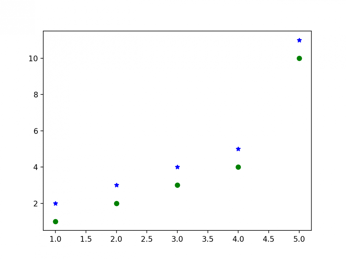
If matplotlib were limited to working with lists, it would be fairlyuseless for numeric processing. Generally, you will use NumPyarrays. In fact, all sequences areconverted to numpy arrays internally. The example below illustrates aplotting several lines with different format styles in one commandusing arrays:
Exercise: Make this plot
Use the plot() documentation to make a plot that looks similar to the oneabove. Start with:
Click to Show/Hide Solution
What are all these icons for?
The figures are enclosed in a window that looks a little like thefollowing(it depends on the OS and matplotlib backend being used):
The icons at the bottom of the window allow you to zoom in or out ofthe plot, pan around, and save the plot as a “hardcopy” format (e.g.PNG, postscript, or PDF).The first icon will reset you to the original axis limits, which comesin quite handy.
You can use the close button to close the window, but it is best touse the close() command to avoid memory leaks.
Saving the plot
As discussed above, you can use the GUI to save the plot, but thesavefig() command is often more useful, and has many options:
Note that you can save a figure multiple times (e.g. as differentformats). The supported formats depend on the backend being used, butnormally include png, pdf, ps, eps and svg:
The default format (used in the first line) can be queried, orchanged, by saying:
Some common-ish Python errors
Here’s a couple of errors you may come across:
Since clf is a function then you need to add () to actuallycall it (being able to refer to a function as a “thing” is incrediblypowerful, which is what has happened here, but it’s not much useif you just want to clear the current figure).
For the second case, x.size returns an integer (in this case5), which we then call as a function, leading to thesomewhat cryptic messsage above. For new users it would be nice if itsaid “hold on, size isn’t callable”, but then this would inhibituseful - if complex - statements such as:
Controlling line properties
What are lines and markers?
A matplotlib “line” is a object containing a set of points and variousattributes describing how to draw those points. The points are optionallydrawn with “markers” and the connections between points can be drawn withvarious styles of line (including no connecting line at all).
Lines have many attributes that you can set: linewidth, dash style,antialiased, etc; see Line2D. There are several ways to set lineproperties
Use keyword args:
Use the setp() command. The example belowuses a MATLAB-style command to set multiple propertieson a list of lines.
setpworks transparently with a list of objectsor a single object:Use the setter methods of the
Line2Dinstance.plotreturns a listof lines; egline1,line2=plot(x1,y1,x2,x2). Below I have onlyone line so it is a list of length 1. I use tuple unpacking in theline,=plot(x,y,'o')to get the first element of the list:Now change the line color, noting that in this case you need to explicitly redraw:
Important
In contrast to old-school plotting where you issue a plot command andthe line is immortalized, in matplotlib the lines (and basically everythingabout the plot) are dynamic objects that can be modified after the fact.
Here are the available Line2D properties.
| Property | Value Type |
|---|---|
| alpha | float |
| animated | [True False] |
| antialiased or aa | [True False] |
| clip_box | a matplotlib.transform.Bbox instance |
| clip_on | [True False] |
| clip_path | a Path instance and a Transform instance, a Patch |
| color or c | any matplotlib color |
| contains | the hit testing function |
| dash_capstyle | [‘butt’ ‘round’ ‘projecting’] |
| dash_joinstyle | [‘miter’ ‘round’ ‘bevel’] |
| dashes | sequence of on/off ink in points |
| data | (array xdata, array ydata) |
| figure | a matplotlib.figure.Figure instance |
| label | any string |
| linestyle or ls | [ ‘-‘ ‘–’ ‘-.’ ‘:’ ‘steps’ ...] |
| linewidth or lw | float value in points |
| lod | [True False] |
| marker | [ ‘+’ ‘,’ ‘.’ ‘1’ ‘2’ ‘3’ ‘4’ ... ] |
| markeredgecolor or mec | any matplotlib color |
| markeredgewidth or mew | float value in points |
| markerfacecolor or mfc | any matplotlib color |
| markersize or ms | float |
| markevery | None integer (startind, stride) |
| picker | used in interactive line selection |
| pickradius | the line pick selection radius |
| solid_capstyle | [‘butt’ ‘round’ ‘projecting’] |
| solid_joinstyle | [‘miter’ ‘round’ ‘bevel’] |
| transform | a matplotlib.transforms.Transform instance |
| visible | [True False] |
| xdata | array |
| ydata | array |
| zorder | any number |
To get a list of settable line properties, call thesetp() function with a line or linesas argument:
Detour into Python
You may have noticed that in the last workshop we mostly used NumPy arrays likenp.arange(5) or np.array([1,2,3,4]) but now you are seeing statements likeplt.plot([1,2,3]).
Multiple Plots Python
Some useful functions for controlling plotting
Here are a few useful functions:
| figure() | Make new figure frame (accepts figsize=(width,height) in inches) |
| autoscale() | Allow or disable autoscaling and control space beyond data limits |
| hold() | Hold figure: hold(False) means next plot() command wipes figure |
| ion(), ioff() | Turn interactive plotting on and off |
| axis() | Set plot axis limits or set aspect ratio (plus more) |
| subplots_adjust() | Adjust the spacing around subplots (fix clipped labels etc) |
| xlim(), ylim() | Set x and y axis limits individually |
| xticks(), yticks() | Set x and y axis ticks |
Working with multiple figures and axes
MATLAB, and matplotlib.pyplot, have the concept of the currentfigure and the current axes. All plotting commands apply to thecurrent axes. The function gca() returns thecurrent axes (an Axes instance), andgcf() returns the current figure(a Figure instance). Normally, you don’t haveto worry about this, because it is all taken care of behind thescenes.
Figure, Axes, plot(), and subplot()
- Figure
- This is the entire window where one or more subplots live.A Figure object (new window) is created with the figure() command.
- Axes
- This is an object representing a subplot (which you might casuallycall a “plot”) which contains axes, ticks, lines, points, text, etc.
- plot()
- This is a command that draws points or lines and returns a list ofLine2D objects. One sublety is that plot() will automaticallycall figure() and/or subplot() if neccesary to create theunderlying Figure and Axes objects.
- subplot()
- This is a command that creates and returns a new subplot (Axes) objectwhich will be used for subsequent plotting commands.
Below is a script that illustrates this by creating two figures where the firstfigure has two subplots:
The first figure() command here is optional becausefigure(1) will be created by default, just as a subplot(1,1,1)will be created by default if you don’t manually specify an axes.
The subplot() command specifies numrows,numcols,fignum wherefignum ranges from 1 to numrows*numcols. The commas in the subplotcommand are optional if numrows*numcols<10 so you might see calls likesubplot(211) in code, but don’t do this yourself. You can create anarbitrary number of subplots and axes.
If you want to place an axes manually, ie, not on a rectangular grid, use theaxes() command, which allows you to specify the location as axes([left,bottom,width,height]) where all values are in fractional (0 to 1)coordinates. See pylab_examples-axes_demofor an example of placing axes manually and pylab_examples-line_stylesfor an example with lots-o-subplots.
You can move back to existing subplots, or indeed figures, as shown below:
You can clear the current figure with clf() and the current axes withcla(). If you find this statefulness, annoying, don’t despair, this is justa thin stateful wrapper around an object oriented API, which you can useinstead. See the Advanced plotting page for an introduction to thisapproach, and the then Artist tutorial for the gory details.
Figures can be deleted with the close() command:
Using close
You can use the ‘close button’ provided by the window managerto remove the figure, but if you do this you must still callthe close() command, to ensure that memory allocated by pyplotfor the figure is released. This is only really an issue forlong-running ipython sessions; if you just create a singleplot and then exit you do not need to use close.
Working with text
The text() command can be used to add text inan arbitrary location, and the xlabel(),ylabel() and title()are used to add text in the indicated locations (see Text introfor a more detailed example):
All of the text() commands return anmatplotlib.text.Text instance. Just as with with linesabove, you can customize the properties by passing keyword argumentsinto the text functions or using setp():
These properties are covered in more detail in text-properties.
Exercise: Overlaying histograms
Make an additional normal distribution with a mean of 130. Make a new plotwhere the two distributions are overlayed. Use a different color andchoose the opacities so it looks reasonable.
Hint:
- You might want to use the
binparameter with anarange(min,max,step)so both histograms are binned the same.
Click to Show/Hide Solution
Getting the fonts just right
The global font properties for various plot elements can be controlled usingthe rc() function:
The inconsistency here is one of the warts in matplotlib. Ironically my favoriteway to find these valuable commands is to google “matplotlib makes mehate”which brings up a blog post ranting about the problems with matplotlib.
All of the attributes that can be controlled with the rc() command arelisted in $HOME/.matplotlib/matplotlibrc and Customizing matplotlib.
See also the Advanced plotting page.
Using mathematical expressions in text
matplotlib accepts TeX equation expressions in any text expression.For example to write the expression in the title,you can write a TeX expression surrounded by dollar signs:
The r preceeding the title string is important – it signifies that thestring is a raw string and not to treate backslashes as python escapes.matplotlib has a built-in TeX expression parser and layout engine, and shipsits own math fonts – for details see the mathtext-tutorial. Thus you can usemathematical text across platforms without requiring a TeX installation. Forthose who have LaTeX and dvipng installed, you can also use LaTeX to formatyour text and incorporate the output directly into your display figures orsaved postscript – see the usetex-tutorial.
Annotating text
The uses of the basic text() command aboveplace text at an arbitrary position on the Axes. A common use case oftext is to annotate some feature of the plot, and theannotate() method provides helperfunctionality to make annotations easy. In an annotation, there aretwo points to consider: the location being annotated represented bythe argument xy and the location of the text xytext. Both ofthese arguments are (x,y) tuples:
In this basic example, both the xy (arrow tip) and xytextlocations (text location) are in data coordinates. There are avariety of other coordinate systems one can choose – see theAnnotations introductionfor more details and links to examples.
Plotting 2-d data
A deeper tutorial on plotting 2-d image data will have to wait for anotherday:
- For simple cases it is straightforward and everything you needto know is in the image tutorial
- For making publication quality images for astronomy you should beusing APLpy.
Plotting 3-d data
Matplotlib supports plotting 3-d data through the mpl_toolkits.mplot3dmodule. This is a somewhat specialized functionality but it’s worth quicklylooking at an example of the 3-d viewer that is available:
To get more information check out the mplot3d tutorial.
Appendix: Pylab and Pyplot and NumPy
You may see examples that use the pylab mode of IPython by usingipython--pylab or the %pylab magic function.Let’s demystify what’s happening in this case andclarify the relationship between pylab and pyplot.
matplotlib.pyplot is a collection of command style functions that makematplotlib work like MATLAB. This is just a package module that you can import:
Likewise pylab is also a module provided by matplotlib that you can import:
This module is a thin wrapper around matplotlib.pylab which pulls in:
- Everything in
matplotlib.pyplot - All top-level functions
numpy,numpy.fft,numpy.random,numpy.linalg - A selection of other useful functions and modules from matplotlib
There is no magic, and to see for yourself do
When you do ipython--pylab it (essentially) just does:
There is one technical detail about GUI event loops and plot window interactionwhich makes it useful to use --pylab even if you are not directly using all thetop-level functions like plot() that get imported.
In a lot of documentation examples you will see code like:
Now you should understand this is the same plot() function that you get inPylab.
2 Plots Python Plot
See Matplotlib, pylab, and pyplot: how are they related?for a more discussion on the topic.
In our previous tutorial, we learned how to plot a straight line, or linear equations of type $y=mx+c$.
Multiple Plots Python Seaborn
Here, we will be learning how to plot a defined function $y=f(x)$ in Python, over a specified interval.
We start off by plotting the simplest quadratic equation $y=x^{2}$.
Python 2 Plots In One Figure
Quadratic Equation
Quadratic equations are second order polynomial equations of type $ax^{2} + bx + c = 0$, where $x$ is a variable and $a ne 0$. Plotting a quadratic function is almost the same as plotting the straight line in the previous tutorial.
Below is the Matplotlib code to plot the function $y=x^{2}$. It is a simple straight-forward code; the bulk of it in the middle is for setting the axes. As the exponent of $x$ is $2$, there will only be positive values of $y$, so we can position ax.spines['bottom'] at the bottom.
2 Axis Python
Cubic Equation
Next, we will plot the simplest cubic function $y=x^{3}$.
Since the exponent in $y=x^{3}$ is $3$, the power is bound to have negative values for negative values of $x$. Therefore, for visibility of negative values in the $y$-axis, we need to move the $x$-axis to the centre of the graph. ax.spines['bottom'] is thus positioned to centre.
Trigonometric Functions
Here we plot the trigonometric function $y=text{sin}(x)$ for the values of $x$ between $-pi$ and $pi$. The linspace() method has its interval set from $-pi$ to $pi$.
Let us plot it together with two more functions, $y=2text{sin}(x)$ and $y=3text{sin}(x)$. This time, we label the functions.
And here we plot together both $y=text{sin}(x)$ and $y=text{cos}(x)$ over the same interval $-pi$ to $pi$.
Exponential Function
The exponential function $y=e^{x}$ is never going to have any negative values for any value of $x$. So we move the $x$-axis to the bottom again by setting ax.spines['bottom'] to zero. We plot it over the interval $-2$ to $2$.